Propagation attenuation with Pycraf

These simulations use the Pycraf module in Python to calculate the propagation attenuation. The relevant pycraf-based scripts can be found in rfi/pycraf_scripts directory. Pycraf utilises the International Telecommunications Union (ITU) recommendation framework and specifically those of ITU-R P.452-16, P.676-10 and F.699-7 that describe the assumed models of the antennas and expected propagation effects. For a full description of the relevant models, please see the ITU documentation.

Propagation

The propagation of the transmission can be affected a number of ways including but not limited to, the effects of the terrain/line-of-sight, diffraction, tropospheric scatter and ducting. The Pycraf module utilises the relevant equations described in ITU-R P.452-16 and P.676-10 from the ITU recommendations to calculate the expected attenuation as a result of these factors between transmitter and receiver.

Terrain data

When calculating the propagation attenuation, the script will automatically download the relevant terrain data from the NASA Shuttle Radar Topography Mission (SRTM) provided by the Jet Propulsion Laboratory. This will be stored by default in the rfi/data/srtm_data directory.

Receivers

For the purposes of modelling the propagation attenuation and simulating the RFI, we are not using a Pycraf-based model of receivers, but rather they are assumed to be represented by the beam-formed station beam. A line-of-sight gain towards the transmitter is calculated for the station beam with OSKAR and used to correct the final propagation model in the next stage.

Simulation inputs

Transmitters

The Pycraf supporting script as well as the main propagation calculation script (see below) can be run using the default input, which represents the basic information for a single transmitter. For the full RFI simulation a CSV file containing information on multiple transmitters is recommended. Information on the digital television antennas in Western Australia is provided (Filtered_DTV_list_plain.csv). This represents a sub-sample of the transmitter information included in the full ACMA (Australian Communications and Media Authority) license list, which also contains more information with regards to each license than is needed for the simulation scripts. Each transmitter in the input CSV should be provided with minimally a name (which will be used alongside the ID to identify the transmitter specific files e.g. attenuation values), a location list (latitude, longitude in degrees), a power [W], a height [m], a central frequency [MHz] and a bandwidth [MHz].

For more information on the transmitter data, see Terrestrial transmitter data.

SKA Low configuration

An input configuration file (txt or equivalent) containing position information in longitude and latitude is necessary to run the main script. By default the Low configuration file used can be found in rfi/data/telescope_files/SKA1-LOW_SKO-0000422_Rev3_38m_SKALA4_spot_frequencies.tm/layout_wgs84.txt.

Calculate propagation attenuation

Propagation attenuation is calculated using SKA_low_RFI_propagation.py. Based on the input information described above, the script will model the transmitters and calculate the expected attenuation at each frequency increment for each requested SKA Low station. Note SKA_low_RFI_propagation.py calls SKA_low_pycraf_propagation.py to perform the core Pycraf calculation.

The attenuation values will then be used to calculate the apparent power of the emitter as an isotropic antenna would see it.

Use of Az/El calculations

When calculating attenuation values that are expected to be used in conjunction with OSKAR beam-gain values (i.e. if using the rfi_sim.sh bash script), it is advisable to use the default setup of --az_calc=True and --non_below_el=True. Though it is possible for signal to be received from a transmitter that is below the horizon to a given station (predominantly via atmospheric effects), OSKAR relies on a horizon limit and will return a beam gain of zero for any transmitters below the horizon. By default, at this stage a line-of-sight calculation is done to find the position of the transmitter with respect to the Low antennas and any transmitters below the horizon are discarded from the simulation. An updated transmitter file in CSV format is written for use in the RASCIL simulation stage. This prevents the simulation of essentially non-contributing transmitters in the final RASCIL script. (Note: it is possible to perform the RASCIL simulation using an input beam gain file or a single value input, which can be used to include these transmitters in the simulated data.)

HDF5 output

The results of the script are written into an HDF5 file, with the structure described at Radio Frequency Interference (RFI) interface. The code will still output all the azimuth-elevation txt files for use in OSKAR. The HDF5 file is the default input for the RASCIL-script. Note: the .hdf5 file can also be the input for the OSKAR-script, but it is not the default behaviour at the moment.

Command line arguments

Pycraf Python script

Pycraf supporting scripts

Within the rfi/pycraf_scripts directory there is an additional script called Test_pycraf_LOW_antenna.py, which is provided to aid with understanding the Pycraf functionality and to enable more comprehensive visualisation of the models and calculations used.

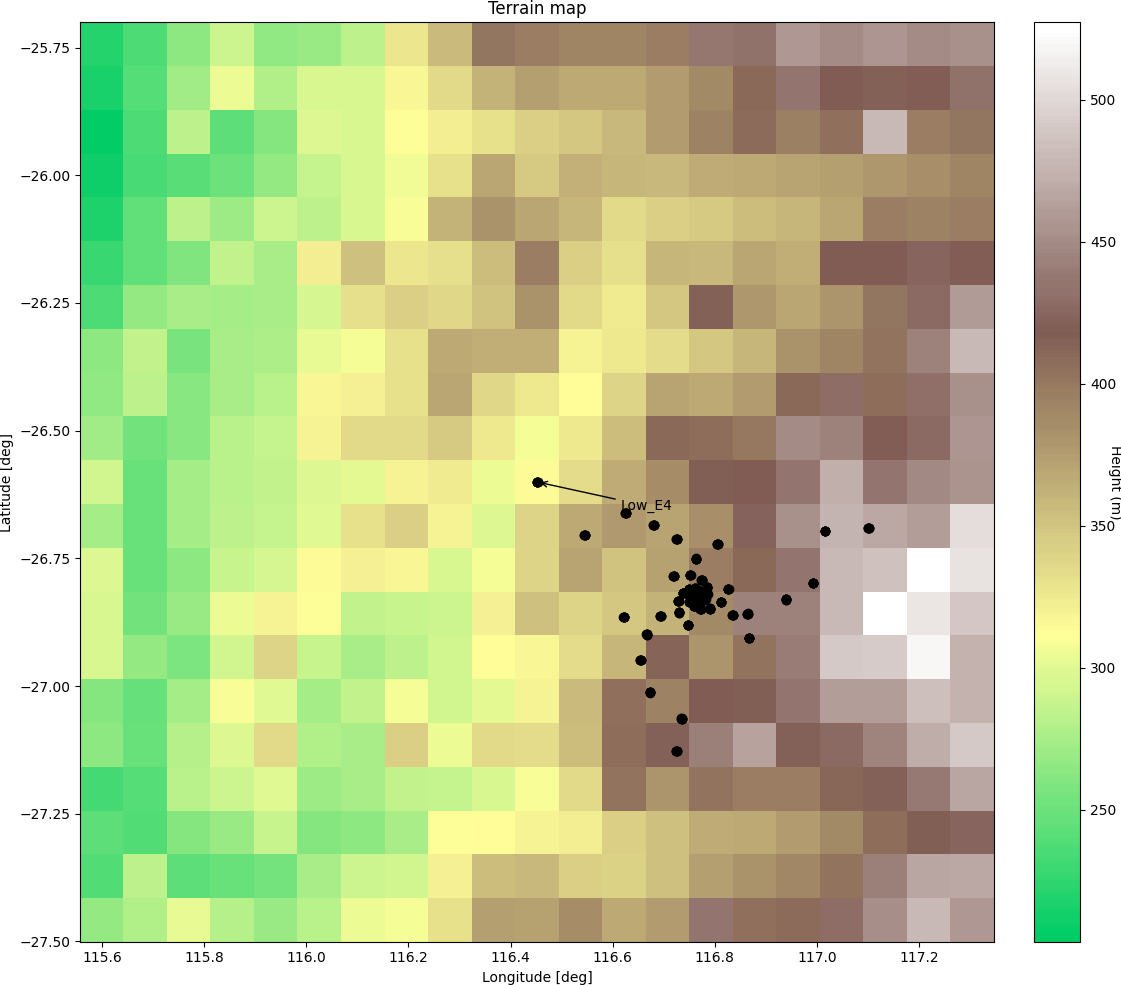
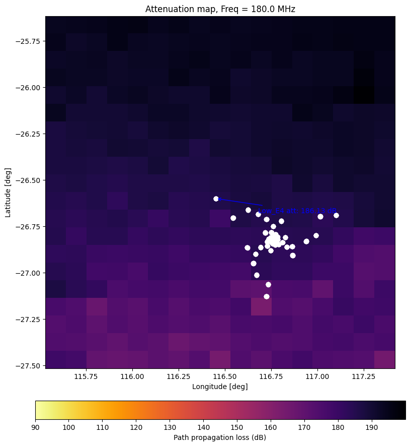
The script is designed to be interactive and the primary input parameters should be easily identifiable within the script itself. This script performs the Pycraf path attenuation calculation for the SKA antennas provided in the SKA Low configuration file (see Simulation inputs for further information). There are additional options to perform and plot a map-based attenuation calculation for visualisation. These can be selected within the code and will produce a map of the relevant SRTM terrain data, a heatmap of the calculated attenuation and a combination of the terrain with overlaid attenuation contours. In each case the positions of the antennas and central array reference point (referred to as ‘LOW_E4’ in the example given) as well as the transmitter (where apppropriate) will be plotted and labelled. The relevant options (do_map_solution, doplotAll and choose_resolution) can be used to limit the images produced to either a small region around the array or the full distance between the array and transmitter. Example outputs are shown below: