Basic concepts
OSKAR provides a toolbox of Python utilities for running simulations, and for making dirty or residual images to analyse the results. Since the potential parameter space for all possible simulations is very large, no single script could sensibly cater for them all - so in order to run a set of simulations for your own investigation, you will probably find it useful to write your own script. Don’t panic though: if you’re familiar with basic Python concepts, this is not hard. Depending on the simulations you want to run and the steps needed to analyse and present the results, the script to drive the simulations could be very simple.
This cookbook outlines some of the key concepts and provides some examples to show what is possible, which could be used as building blocks for your own scripts.
As shown in the sketch below, to produce simulated visibilities, OSKAR needs as inputs a sky model, a telescope model, and a few parameters to describe the observation.
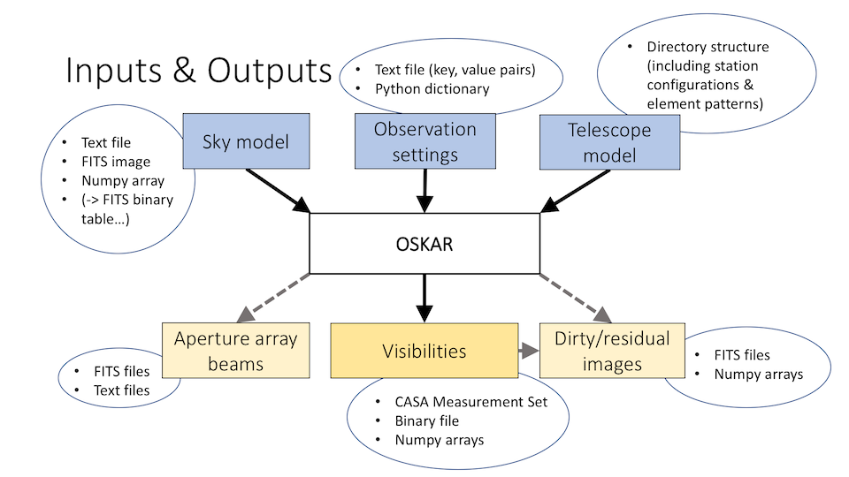
Overview of OSKAR inputs and outputs
Any simulation script will usually need to iterate over a number of simulated observations, changing parts of the sky model, the telescope model and/or the parameters in a systematic way for each run. Ways to set up the sky model and the telescope model are described on later pages, but the most commonly used settings parameters are outlined below.
Commonly used settings
The settings parameters used by OSKAR are generated from a Python dictionary of key-value pairs.
The following parameters will almost always need to be set appropriately when running any interferometer simulation with OSKAR. The values given below are examples only!
params = {
    'simulator': {
        'use_gpus': True  # or False
    },
    'observation': {
        'num_channels': 3,  # Simulate 3 frequency channels
        'start_frequency_hz': 100e6,  # First channel at 100 MHz
        'frequency_inc_hz': 20e6,  # Channel separation of 20 MHz
        'phase_centre_ra_deg': 20,
        'phase_centre_dec_deg': -30,
        'num_time_steps': 24,  # Simulate 24 correlator dumps
        'start_time_utc': '2000-01-01 12:00:00.000',
        'length': '12:00:00.000'  # 12 hours, or length in seconds
    },
    'telescope': {
        'input_directory': '/absolute/or/relative/path/to/a/telescope_model_folder.tm/'
    },
    'interferometer': {
        'channel_bandwidth_hz': 10e3,
        'time_average_sec': 1.0,
        'oskar_vis_filename': 'example.vis',
        'ms_filename': 'example.ms'
    }
}
The dictionary keys may be nested, as above, or flat if it is more convenient. The following is entirely equivalent to the above:
params = {
    'simulator/use_gpus': True,  # or False
    'observation/num_channels': 3,  # Simulate 3 frequency channels
    'observation/start_frequency_hz': 100e6,  # First channel at 100 MHz
    'observation/frequency_inc_hz': 20e6,  # Channel separation of 20 MHz
    'observation/phase_centre_ra_deg': 20,
    'observation/phase_centre_dec_deg': -30,
    'observation/num_time_steps': 24,  # Simulate 24 correlator dumps
    'observation/start_time_utc': '2000-01-01 12:00:00.000',
    'observation/length': '12:00:00.000',  # 12 hours, or length in seconds
    'telescope/input_directory': '/absolute/or/relative/path/to/a/telescope_model_folder.tm/',
    'interferometer/channel_bandwidth_hz': 10e3,
    'interferometer/time_average_sec': 1.0,
    'interferometer/oskar_vis_filename': 'example.vis',
    'interferometer/ms_filename': 'example.ms'
}
Using these example parameters, simulated visibility data will be written to
a CASA Measurement Set specified by the interferometer/ms_filename
settings key (in this case example.ms) and also a binary visibility
data file specified by the interferometer/oskar_vis_filename key
(here, example.vis).
Most of the rest of the parameters specify the time and frequency coverage of the observation, as well as the direction of the phase centre.
The hardest parameter to set is usually the start time.
To help with this, a utility function called get_start_time is provided
in the file utils.py, which calculates an optimal start time using the
target Right Ascension, the observation length, and the longitude of the
SKA-Low telescope. The observation will then be symmetric about the meridian.
The full list of settings parameters is shown in the OSKAR GUI for the
oskar_sim_interferometer application, and also in the
settings documentation.
Creating a settings tree and interferometer simulator
After defining parameters in a standard Python dictionary as above, an OSKAR
SettingsTree should be created from it, and this can be used to instantiate
other classes to run a simulation.
To set up an oskar.Interferometer simulator in Python, use the parameters
for the oskar_sim_interferometer application, and then set them from the
Python dictionary as follows:
settings = oskar.SettingsTree('oskar_sim_interferometer')
settings.from_dict(params)  # using the Python dictionary above.
This settings object can then be passed as a parameter to the constructor:
sim = oskar.Interferometer(settings=settings)
Setting the input data models
A sky model and telescope model can be defined either using the settings
parameters, or set programmatically from Python - the latter option
being useful, for example, if changing a model within a loop. The methods
oskar.Interferometer.set_sky_model() and
oskar.Interferometer.set_telescope_model() can be used for this.
See the following pages for more details.